Microsoft Excel is a spreadsheet program that contains one or more worksheets. Each worksheet contains a bunch of cells which are located by a row (1,2,3,etc) and a column (A,B,C,etc).
Each cell can contain data or a formula. With a formula your able to transform the data from other cells to whatever you may need. You’ll probably want to re-use the formula in different rows, columns or worksheets.
A formula contains a function (like min, max, average, etc) and a range of data (like A:A or A1:A10).
For example I’ve filled row 1 to 10 on column A with the corresponding numbers. In Cell B1 we’ve created a formula that calculates the average of these 10 cells : =AVERAGE(A1:A10).
PS: The screenshot says ‘gemiddelde’ which is Dutch for average.
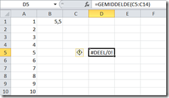
Now we copy the content of cell B1, which contains the formula, and copy it to cell D5.
The result of cell D5 is “division by zero”. When we look at the formula we see that Microsoft Excel transformed both the column and the row corresponding to the location where we moved it (+2 columns, +4 rows).
Altough this might be usefull in some cases, in some cases it isn’t.
There is a little trick which helps you setting constraints when copying formula’s. The use of the $ sign. If you place a $ sign in front of a column or a row it will become static. It won’t be transformed when you copy the content of a cell.
Let’s take a look at how this works.
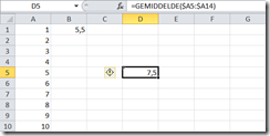
When we change the content of cell B1 to =AVERAGE($A1:$A10) where setting a constraint on the row, row A is now static. When we copy the cell to D5 the formula in D5 will be =AVERAGE($A5:$A14).
When we repeat the same thing but instead of setting a constraint on the row we’re setting a constraint on the column. The content of cell B1 will be = AVERAGE(A$1:A$10).
Now the formula in cell D5 will be =AVERAGE(C$1:C$10). The column is changed, but the row’s are not.
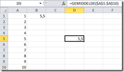
Now let’s set a constraint on the formula in cell B1 where we make both the column and the row static. The content of cell B1 is =AVERAGE($A$1:$A$10). After copying cell B1 to D5 the both the formula and the result of cell D5 matches B1:
Although it’s very simple and looks non-trivial, the little things like this makes my live a lot easier when working with formulas in Excel.
Ingmar Verheij


